This is a companion post to my IGL article. There, I teased “AtlasBlock for Language Models” as a future direction. This post is that future — I decided over the weekend to give a try to OpenAI’s Parameter Golf Challenge with IGL, building MHALM (Multi-Head Atlas Language Model), a language model entirely on IGL’s geometric kernel framework. The goal was not to win but to stress-test whether IGL’s ideas could work at all for token prediction. They can.
The Parameter Golf Challenge
OpenAI’s Parameter Golf is a competition with brutal constraints: build the best language model within a 16 MB artifact, trained in 10 minutes on 8×H100 GPUs, evaluated on FineWeb using bits-per-byte (bpb) — lower is better.
OpenAI provides a baseline — a 9-layer decoder-only transformer (d=512, V=1024, context 1024) with grouped-query attention (8 heads, 4 KV heads). Looking at the current submission track, most entries focus on engineering tricks to squeeze more performance out of transformer variants. My goal was different: leverage IGL to build a fundamentally different architecture and see how close it could get to the baseline.
The Core Idea: From Green’s Functions to Token Prediction
IGL in a Nutshell
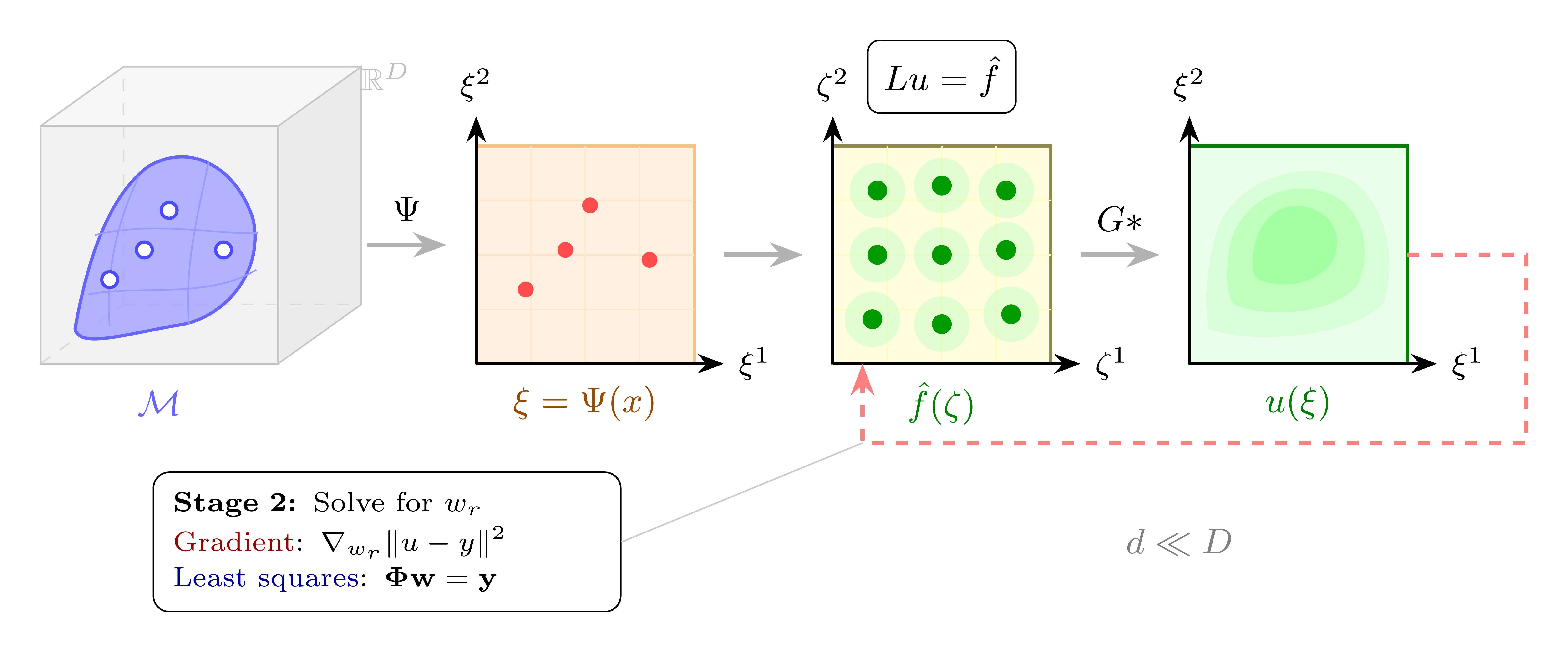
The Intrinsic Green’s Learning (IGL) framework starts from the manifold hypothesis: data lives on a low-dimensional manifold \(\mathcal{M} \subset \mathbb{R}^D\), with intrinsic dimension \(d \ll D\). Rather than letting a network discover this structure implicitly, IGL bakes it into the architecture.
The core idea is to frame the target function \(u\) as the solution to a linear PDE: \(Lu = f\), where \(L\) is a differential operator and \(f\) is a learned source term. The solution is given by convolution with the Green’s function: \(u(\xi) = \int G(\xi, \zeta) f(\zeta) \, d\zeta\). This is not a physical claim — it is an architectural choice that buys a crucial property: linearity in the source weights. Once an encoder \(\Psi\) maps data to intrinsic coordinates \(\xi\), finding the optimal source reduces to linear least squares.
In practice, this yields a three-step pipeline: (1) an encoder \(\Psi\) maps input \(x \in \mathbb{R}^D\) to intrinsic coordinates \(\xi \in \mathbb{R}^d\), (2) a kernel basis \(\Phi(\xi)\) is evaluated — this is where the Green’s function structure lives — and (3) a readout matrix \(W\) maps \(\Phi\) to predictions. The kernel generates large effective weight matrices on the fly from compact parameters, which is where the compression comes from.
See the companion article for the full derivation.
From Manifolds to Token Embeddings
How does this apply to language modelling? In Parameter Golf, the vocabulary has \(V = 1024\) tokens embedded in \(\mathbb{R}^{512}\). These token embeddings form a discrete manifold — a structured point cloud with geometric regularity that IGL can exploit. An encoder \(\Psi\) maps token embeddings to intrinsic coordinates; different kernel bases capture different geometric aspects of this token manifold. Figure 2 illustrates the mapping and how MHALM extends IGL’s single chart to multiple complementary charts.
The Parameter Budget Argument
In a standard LM, the output projection \(W \in \mathbb{R}^{d \times V}\) maps hidden states to vocabulary logits. For \(V = 1024\) and \(d = 256\), that’s 262K parameters per head — and MHALM has 5 heads × 2 blocks. Storing all these \(W\) matrices would consume ~12 MB of the 16 MB budget. IGL’s kernel structure keeps the design matrices \(\Phi\) compact, while the readout matrices \(W\) are trained end-to-end as learned readout matrices.
This naturally leads to the name: in topology, an atlas is a collection of charts that together describe a manifold — each chart maps a region to coordinates. In this case, the name is admittedly a bit of a misnomer: the charts don’t cover different regions of the token manifold, but capture different geometric properties of the same manifold — angular structure (Spherical), oscillatory patterns (Gabor), and proximity (Laplacian). Multiple complementary coordinate systems, each revealing structure the others miss. Instead of one monolithic attention mechanism, our architecture uses multiple geometric kernel heads, each computing a different view of the embedding space, then combining their predictions.
The Architecture
The resulting architecture — the Multi-Head Atlas Language Model (MHALM) — replaces transformer attention with a multi-kernel geometric readout. The core building block is the HybridAtlasBlock: five kernel heads that each compute a different geometric view of the token manifold, combined by a learned mixer, then processed by a temporal stack. Two such blocks, stacked with a skip connection, form the full model.
The HybridAtlasBlock
The Encoders (Charts)
Three independent MLP encoders map token embeddings to intrinsic coordinates — each one a chart on the token manifold. Their widths are asymmetric, matched to the complexity of the kernel they feed:
- \(\Psi_0\) (H=700): the widest encoder, feeds the Spherical head.
- \(\Psi_1\) (H=256): feeds the Gabor head.
- \(\Psi_2\) (H=384): feeds the Laplacian head.
These widths were chosen by rough trial and error under time pressure — a more systematic search over encoder capacities is needed.
These are the charts of the atlas — three independent coordinate systems, each specialised for a different geometric structure. A Stäckel separability penalty (\(\beta \cdot \|\text{off-diag}(\text{Cov}(z))\|^2\)) encourages the encoded coordinates to be geometrically independent across axes — the discrete analogue of a Stäckel separable Laplace-Beltrami operator.
The Five Kernel Heads
Each head takes encoder output (or raw input) and produces vocabulary logits through a different kernel family:
Spherical head. Encoder \(\Psi_0\) maps tokens to coordinates \(z_0\). A Nyström causal kernel with 256 landmarks approximates a large kernel matrix without materialising it — computing \(\Phi_0(z_0)\) as a low-rank factorisation. The readout \(W_0\) maps \(\Phi_0\) to logits. Unlike the other heads, the Spherical head doesn’t correspond to a single PDE operator — it approximates a causal token-to-token kernel using landmark positions, with a learnable Gegenbauer polynomial mixture. Gegenbauer polynomials \(C_n^{(\alpha)}\) are the natural basis for zonal functions on the sphere \(S^{d-1}\) — they generalise Legendre polynomials to arbitrary dimension and form an orthogonal basis for functions of the cosine angle between two vectors. Using a learned mixture of Gegenbauer polynomials lets the kernel express arbitrary angular similarity profiles beyond simple cosine similarity. Where Gabor and Laplacian operate in encoder coordinate space (anchor-to-token), the Spherical head operates in token-to-token space (position-to-position), making it structurally closer to attention.
Gabor head. Encoder \(\Psi_1\) maps tokens to coordinates \(z_1\). A Gabor basis evaluates \(\Phi_1(z_1)\) against \(R=128\) learned anchors. In the IGL framework, this corresponds to the Helmholtz operator \(-\Delta + \kappa^2 I\) with Gaussian window: the Green’s function of the Helmholtz equation produces localised oscillatory responses — Gabor wavelets \(\phi(z) = \exp(-\|z-\mu\|^2 / 2\sigma^2) \cdot \cos(k^\top z + \varphi)\). Each basis function is a localised oscillation centred at an anchor point, capturing frequency-like patterns — features that are both localised in space and have a characteristic frequency. The readout \(W_1\) maps \(\Phi_1\) to logits.
Laplacian head. Encoder \(\Psi_2\) maps tokens to coordinates \(z_2\). An RBF mixture with \(R=128\) learned anchors evaluates \(\Phi_2(z_2)\). This corresponds to the negative Laplacian \(-\Delta\) — the heat kernel / Poisson equation. The Green’s function is a radial basis function: \(\phi(z) = \exp(-\|z-\mu\|^2 / 2\sigma^2)\). This is the original IGL basis, the most thoroughly validated family. It captures smooth, global proximity structure: tokens close in encoder space get similar kernel responses. The readout \(W_2\) maps \(\Phi_2\) to logits.
Tucker GL head. No dedicated encoder — this head takes the Hadamard product \(\Phi_1 \odot \Phi_2\) of the Gabor and Laplacian bases. In PDE terms, this is an operator product — the conjunction of Helmholtz (oscillatory) and Laplacian (proximity) structure. The Hadamard product of two separable kernels is itself separable, so the tensor structure is preserved. This is a Tucker decomposition of the joint kernel, capturing geometric conjunctions (“oscillatory and proximate”) that neither basis alone can represent. Crucially, this head is essentially parameter-free beyond its readout: it reuses \(\Phi_1\) and \(\Phi_2\) already computed by the Gabor and Laplacian heads, adding model expressivity at near-zero cost. The readout \(W_3\) maps the product to logits.
Linear head. No encoder, no kernel — takes the raw input \(x\) directly and maps it through \(W_4\) to logits. In PDE terms, this is the identity operator \(L = I\), where \(G = \delta\) — the “kernel basis” is just the raw input itself. This serves as a baseline: if the embedding already carries useful structure, a simple linear readout should capture it. The fact that it contributes meaningfully (removing it costs +0.04 nats) suggests the embedding learns useful representations even without geometric processing.
HeadScaler and Temporal Processing
A HeadScaler combines the five logit tensors with learned softmax weights: \(\text{mixed} = \sum_k \text{softmax}(\alpha_k) \cdot \text{softcap}(\text{logits}_k)\). The softcap prevents any single head from dominating early in training.
The mixed logits then pass through the temporal stack:
- ComplexSSM — a state-space model with complex eigenvalues (\(h_t = e^{\lambda + i\omega} \cdot h_{t-1} + u_t\)), implemented via parallel scan. This captures long-range temporal dependencies at O(T) cost, inspired by Mamba-2.
- CausalSelfAttention ×2 — two layers of standard causal attention with RoPE positional encoding, 8 heads, and query gain. A residual skip connects the SSM output to the attention output.
A Note on Dimension Discovery
In the IGL framework, Matryoshka truncation can be used to discover the effective dimension each kernel needs: during training, each head randomly samples \(k_m \sim \text{Uniform}\{1, \ldots, d_{\max}\}\) and truncates to that dimension, producing nested representations. This was tested early on and worked well (zero collapse failures, unlike Hard Concrete gates). However, for the competition submission, dimension discovery was removed — knowing the optimal per-head dimension is valuable for research but costs FLOPS at inference, and the challenge rewards raw bpb, not interpretability.
The Full Model
Two HybridAtlasBlocks are stacked to form the complete MHALM architecture (Figure 4):
- Embedding + BigramHash — a weight-tied embedding \(E \in \mathbb{R}^{V \times d_{\text{emb}}}\) maps tokens to vectors, augmented with a bigram hash for local context.
- HybridAtlasBlock 0 — the first block processes the embedded tokens through its five heads and temporal stack.
- U-Net skip connection — the encoder outputs (\(z_0, z_1, z_2\)) from Block 0 are projected and added to the block’s output, providing a direct path for geometric information.
- HybridAtlasBlock 1 — the second block, with independent weights, refines the representation.
- Output projection — \(\text{softcap}(W_{\text{out}} \cdot H \cdot E^\top)\) produces final logits, reusing the embedding matrix \(E\) (weight tying).
Results
| Metric | Value |
|---|---|
| Competition bpb | 1.4574 |
| Val loss (nats) | 2.4607 |
| Artifact size | 10.8 MB / 16 MB |
| Stored params | 13.6M |
| Training steps | 6,857 |
| Training time | 594s on 8×H100 |
| Step time (compiled) | 87 ms/step |
| SWA checkpoints | 201 |
📋 Full training log (v1)
FineWeb: 80 train shards, 1 val shards
train_loader:dataset:fineweb10B_sp1024 train_shards:80
val_loader:tokens:62021846
val_bpb:enabled tokenizer_kind=sentencepiece tokenizer_path=/workspace/parameter-golf/data/tokenizers/fineweb_1024_bpe.model
model_params:13631099
world_size:8 train_batch_tokens:524288 train_seq_len:1024 max_wallclock_seconds:600.000
architecture:MHALM L=2 H=700 R=128 R_s=128 bigram_vocab=10240
step:50/5940 train_loss:5.1160 train_time:42809ms step_avg:856.18ms
step:100/5940 train_loss:4.4082 train_time:46631ms step_avg:466.31ms
step:150/5940 train_loss:3.9050 train_time:50458ms step_avg:336.39ms
step:200/5940 train_loss:3.6059 train_time:54305ms step_avg:271.52ms
step:200/5940 val_loss:3.6478 val_bpb:5.2626 est_bpb:2.1568 train_time:71312ms step_avg:356.56ms
step:250/5940 train_loss:3.4682 train_time:75147ms step_avg:300.59ms
step:300/5940 train_loss:3.3736 train_time:78978ms step_avg:263.26ms
step:350/5940 train_loss:3.3056 train_time:83467ms step_avg:238.48ms
step:400/5940 train_loss:3.2089 train_time:87299ms step_avg:218.25ms
step:400/5940 val_loss:3.2268 val_bpb:4.6552 est_bpb:1.9079 train_time:87518ms step_avg:218.79ms
  Refined: 81 ms/step → est_total=6652
step:450/6652 train_loss:3.2282 train_time:91347ms step_avg:202.99ms
step:500/6652 train_loss:3.1729 train_time:95170ms step_avg:190.34ms
step:550/6652 train_loss:3.0824 train_time:98996ms step_avg:179.99ms
step:600/6652 train_loss:3.0977 train_time:102827ms step_avg:171.38ms
step:600/6652 val_loss:3.0833 val_bpb:4.4483 est_bpb:1.8231 train_time:103047ms step_avg:171.75ms
step:650/6652 train_loss:3.1019 train_time:106873ms step_avg:164.42ms
step:700/6652 train_loss:3.0062 train_time:110709ms step_avg:158.16ms
step:750/6652 train_loss:3.1286 train_time:114549ms step_avg:152.73ms
step:800/6652 train_loss:3.0584 train_time:118387ms step_avg:147.98ms
step:800/6652 val_loss:2.9894 val_bpb:4.3128 est_bpb:1.7676 train_time:118606ms step_avg:148.26ms
step:850/6652 train_loss:2.9202 train_time:122442ms step_avg:144.05ms
step:900/6652 train_loss:2.9602 train_time:126283ms step_avg:140.31ms
step:950/6652 train_loss:2.9743 train_time:130121ms step_avg:136.97ms
step:1000/6652 train_loss:2.8816 train_time:133958ms step_avg:133.96ms
step:1000/6652 val_loss:2.9333 val_bpb:4.2318 est_bpb:1.7344 train_time:134178ms step_avg:134.18ms
step:1050/6652 train_loss:2.9228 train_time:138019ms step_avg:131.45ms
step:1100/6652 train_loss:2.9035 train_time:141868ms step_avg:128.97ms
step:1150/6652 train_loss:2.8642 train_time:145711ms step_avg:126.71ms
step:1200/6652 train_loss:2.8431 train_time:149635ms step_avg:124.70ms
step:1200/6652 val_loss:2.8907 val_bpb:4.1705 est_bpb:1.7092 train_time:149853ms step_avg:124.88ms
step:1250/6652 train_loss:2.8910 train_time:153697ms step_avg:122.96ms
step:1300/6652 train_loss:2.8959 train_time:157536ms step_avg:121.18ms
step:1350/6652 train_loss:2.8669 train_time:161373ms step_avg:119.54ms
step:1400/6652 train_loss:2.8688 train_time:165213ms step_avg:118.01ms
step:1400/6652 val_loss:2.8587 val_bpb:4.1243 est_bpb:1.6903 train_time:165431ms step_avg:118.17ms
step:1450/6652 train_loss:2.8232 train_time:169269ms step_avg:116.74ms
step:1500/6652 train_loss:2.8378 train_time:173115ms step_avg:115.41ms
step:1550/6652 train_loss:2.8369 train_time:177332ms step_avg:114.41ms
step:1600/6652 train_loss:2.8903 train_time:181162ms step_avg:113.23ms
step:1600/6652 val_loss:2.8317 val_bpb:4.0853 est_bpb:1.6743 train_time:181380ms step_avg:113.36ms
step:1650/6652 train_loss:2.8032 train_time:185203ms step_avg:112.24ms
step:1700/6652 train_loss:2.8109 train_time:189031ms step_avg:111.19ms
step:1750/6652 train_loss:2.8637 train_time:192859ms step_avg:110.21ms
step:1800/6652 train_loss:2.8606 train_time:196685ms step_avg:109.27ms
step:1800/6652 val_loss:2.7987 val_bpb:4.0377 est_bpb:1.6548 train_time:196905ms step_avg:109.39ms
step:1850/6652 train_loss:2.7811 train_time:200734ms step_avg:108.50ms
step:1900/6652 train_loss:2.7883 train_time:204563ms step_avg:107.66ms
step:1950/6652 train_loss:2.7400 train_time:208396ms step_avg:106.87ms
step:2000/6652 train_loss:2.7773 train_time:212224ms step_avg:106.11ms
step:2000/6652 val_loss:2.7707 val_bpb:3.9973 est_bpb:1.6382 train_time:212442ms step_avg:106.22ms
step:2050/6652 train_loss:2.7165 train_time:216271ms step_avg:105.50ms
step:2100/6652 train_loss:2.7933 train_time:220103ms step_avg:104.81ms
step:2150/6652 train_loss:2.7398 train_time:223931ms step_avg:104.15ms
step:2200/6652 train_loss:2.7860 train_time:227759ms step_avg:103.53ms
step:2200/6652 val_loss:2.7322 val_bpb:3.9417 est_bpb:1.6155 train_time:227979ms step_avg:103.63ms
step:2250/6652 train_loss:2.7376 train_time:231809ms step_avg:103.03ms
step:2300/6652 train_loss:2.6855 train_time:235639ms step_avg:102.45ms
step:2350/6652 train_loss:2.7192 train_time:239467ms step_avg:101.90ms
step:2400/6652 train_loss:2.6708 train_time:243298ms step_avg:101.37ms
step:2400/6652 val_loss:2.7013 val_bpb:3.8971 est_bpb:1.5972 train_time:243516ms step_avg:101.47ms
step:2450/6652 train_loss:2.6720 train_time:247346ms step_avg:100.96ms
step:2500/6652 train_loss:2.7050 train_time:251174ms step_avg:100.47ms
step:2550/6652 train_loss:2.6407 train_time:255004ms step_avg:100.00ms
step:2600/6652 train_loss:2.6422 train_time:258836ms step_avg:99.55ms
step:2600/6652 val_loss:2.6716 val_bpb:3.8543 est_bpb:1.5796 train_time:259054ms step_avg:99.64ms
step:2650/6652 train_loss:2.6318 train_time:262882ms step_avg:99.20ms
step:2700/6652 train_loss:2.7187 train_time:266715ms step_avg:98.78ms
step:2750/6652 train_loss:2.6519 train_time:270558ms step_avg:98.38ms
step:2800/6652 train_loss:2.6581 train_time:274403ms step_avg:98.00ms
step:2800/6652 val_loss:2.6463 val_bpb:3.8178 est_bpb:1.5647 train_time:274621ms step_avg:98.08ms
step:2850/6652 train_loss:2.6416 train_time:278456ms step_avg:97.70ms
step:2900/6652 train_loss:2.6657 train_time:282297ms step_avg:97.34ms
step:2950/6652 train_loss:2.6675 train_time:286133ms step_avg:96.99ms
step:3000/6652 train_loss:2.6363 train_time:289968ms step_avg:96.66ms
step:3000/6652 val_loss:2.6187 val_bpb:3.7779 est_bpb:1.5483 train_time:290187ms step_avg:96.73ms
step:3050/6652 train_loss:2.5439 train_time:294032ms step_avg:96.40ms
step:3100/6652 train_loss:2.6148 train_time:298224ms step_avg:96.20ms
step:3150/6652 train_loss:2.5663 train_time:302057ms step_avg:95.89ms
step:3200/6652 train_loss:2.6009 train_time:305888ms step_avg:95.59ms
step:3200/6652 val_loss:2.5937 val_bpb:3.7420 est_bpb:1.5336 train_time:306105ms step_avg:95.66ms
step:3250/6652 train_loss:2.5873 train_time:309935ms step_avg:95.36ms
step:3300/6652 train_loss:2.6085 train_time:313767ms step_avg:95.08ms
step:3350/6652 train_loss:2.6770 train_time:317596ms step_avg:94.80ms
step:3400/6652 train_loss:2.5753 train_time:321428ms step_avg:94.54ms
step:3400/6652 val_loss:2.5850 val_bpb:3.7294 est_bpb:1.5284 train_time:321645ms step_avg:94.60ms
step:3450/6652 train_loss:2.6232 train_time:325471ms step_avg:94.34ms
step:3500/6652 train_loss:2.5399 train_time:329305ms step_avg:94.09ms
step:3550/6652 train_loss:2.5382 train_time:333137ms step_avg:93.84ms
step:3600/6652 train_loss:2.5801 train_time:336964ms step_avg:93.60ms
step:3600/6652 val_loss:2.5629 val_bpb:3.6975 est_bpb:1.5154 train_time:337182ms step_avg:93.66ms
step:3650/6652 train_loss:2.5886 train_time:341013ms step_avg:93.43ms
step:3700/6652 train_loss:2.5715 train_time:344838ms step_avg:93.20ms
step:3750/6652 train_loss:2.5622 train_time:348667ms step_avg:92.98ms
step:3800/6652 train_loss:2.5529 train_time:352496ms step_avg:92.76ms
step:3800/6652 val_loss:2.5505 val_bpb:3.6796 est_bpb:1.5080 train_time:352714ms step_avg:92.82ms
step:3850/6652 train_loss:2.5438 train_time:356542ms step_avg:92.61ms
step:3900/6652 train_loss:2.5986 train_time:360445ms step_avg:92.42ms
step:3950/6652 train_loss:2.5702 train_time:364312ms step_avg:92.23ms
step:4000/6652 train_loss:2.5410 train_time:368181ms step_avg:92.05ms
step:4000/6652 val_loss:2.5379 val_bpb:3.6614 est_bpb:1.5006 train_time:368399ms step_avg:92.10ms
step:4050/6652 train_loss:2.5595 train_time:372284ms step_avg:91.92ms
step:4100/6652 train_loss:2.5386 train_time:376152ms step_avg:91.74ms
step:4150/6652 train_loss:2.4298 train_time:380032ms step_avg:91.57ms
step:4200/6652 train_loss:2.4827 train_time:383922ms step_avg:91.41ms
step:4200/6652 val_loss:2.5262 val_bpb:3.6445 est_bpb:1.4936 train_time:384352ms step_avg:91.51ms
step:4250/6652 train_loss:2.5405 train_time:388231ms step_avg:91.35ms
step:4300/6652 train_loss:2.5484 train_time:392101ms step_avg:91.19ms
step:4350/6652 train_loss:2.4827 train_time:395983ms step_avg:91.03ms
step:4400/6652 train_loss:2.4675 train_time:399849ms step_avg:90.87ms
step:4400/6652 val_loss:2.5104 val_bpb:3.6218 est_bpb:1.4843 train_time:400065ms step_avg:90.92ms
step:4450/6652 train_loss:2.4926 train_time:403933ms step_avg:90.77ms
step:4500/6652 train_loss:2.5089 train_time:407827ms step_avg:90.63ms
step:4550/6652 train_loss:2.5015 train_time:411693ms step_avg:90.48ms
step:4600/6652 train_loss:2.5078 train_time:415919ms step_avg:90.42ms
step:4600/6652 val_loss:2.5102 val_bpb:3.6214 est_bpb:1.4842 train_time:416136ms step_avg:90.46ms
step:4650/6652 train_loss:2.5209 train_time:420017ms step_avg:90.33ms
step:4700/6652 train_loss:2.4790 train_time:423885ms step_avg:90.19ms
step:4750/6652 train_loss:2.4991 train_time:427751ms step_avg:90.05ms
step:4800/6652 train_loss:2.5007 train_time:431634ms step_avg:89.92ms
step:4800/6652 val_loss:2.4971 val_bpb:3.6025 est_bpb:1.4764 train_time:431847ms step_avg:89.97ms
step:4850/6652 train_loss:2.5201 train_time:435714ms step_avg:89.84ms
step:4900/6652 train_loss:2.4749 train_time:439580ms step_avg:89.71ms
step:4950/6652 train_loss:2.4810 train_time:443466ms step_avg:89.59ms
step:5000/6652 train_loss:2.4619 train_time:447332ms step_avg:89.47ms
step:5000/6652 val_loss:2.4851 val_bpb:3.5853 est_bpb:1.4694 train_time:447760ms step_avg:89.55ms
step:5050/6652 train_loss:2.4520 train_time:451627ms step_avg:89.43ms
step:5100/6652 train_loss:2.4890 train_time:455510ms step_avg:89.32ms
step:5150/6652 train_loss:2.4227 train_time:459376ms step_avg:89.20ms
step:5200/6652 train_loss:2.5266 train_time:463241ms step_avg:89.08ms
step:5200/6652 val_loss:2.4833 val_bpb:3.5826 est_bpb:1.4683 train_time:463458ms step_avg:89.13ms
step:5250/6652 train_loss:2.5109 train_time:467339ms step_avg:89.02ms
step:5300/6652 train_loss:2.5179 train_time:471206ms step_avg:88.91ms
step:5350/6652 train_loss:2.5262 train_time:475072ms step_avg:88.80ms
step:5400/6652 train_loss:2.4881 train_time:478954ms step_avg:88.70ms
step:5400/6652 val_loss:2.4820 val_bpb:3.5807 est_bpb:1.4675 train_time:479169ms step_avg:88.73ms
step:5450/6652 train_loss:2.4434 train_time:483034ms step_avg:88.63ms
step:5500/6652 train_loss:2.4327 train_time:486902ms step_avg:88.53ms
step:5550/6652 train_loss:2.4115 train_time:490784ms step_avg:88.43ms
step:5600/6652 train_loss:2.4591 train_time:494649ms step_avg:88.33ms
step:5600/6652 val_loss:2.4751 val_bpb:3.5708 est_bpb:1.4635 train_time:494865ms step_avg:88.37ms
step:5650/6652 train_loss:2.4178 train_time:498732ms step_avg:88.27ms
step:5700/6652 train_loss:2.5184 train_time:502617ms step_avg:88.18ms
step:5750/6652 train_loss:2.5329 train_time:506486ms step_avg:88.08ms
step:5800/6652 train_loss:2.4388 train_time:510363ms step_avg:87.99ms
step:5800/6652 val_loss:2.4706 val_bpb:3.5643 est_bpb:1.4608 train_time:510580ms step_avg:88.03ms
step:5850/6652 train_loss:2.3956 train_time:514465ms step_avg:87.94ms
step:5900/6652 train_loss:2.4696 train_time:518337ms step_avg:87.85ms
step:5950/6652 train_loss:2.4395 train_time:522208ms step_avg:87.77ms
step:6000/6652 train_loss:2.4357 train_time:526093ms step_avg:87.68ms
step:6000/6652 val_loss:2.4624 val_bpb:3.5526 est_bpb:1.4560 train_time:526306ms step_avg:87.72ms
step:6050/6652 train_loss:2.4417 train_time:530190ms step_avg:87.63ms
step:6100/6652 train_loss:2.3727 train_time:534061ms step_avg:87.55ms
step:6150/6652 train_loss:2.4610 train_time:538339ms step_avg:87.53ms
step:6200/6652 train_loss:2.4728 train_time:542210ms step_avg:87.45ms
step:6200/6652 val_loss:2.4590 val_bpb:3.5475 est_bpb:1.4539 train_time:542427ms step_avg:87.49ms
step:6250/6652 train_loss:2.4487 train_time:546297ms step_avg:87.41ms
step:6300/6652 train_loss:2.4478 train_time:550195ms step_avg:87.33ms
step:6350/6652 train_loss:2.4534 train_time:554064ms step_avg:87.25ms
step:6400/6652 train_loss:2.4868 train_time:557931ms step_avg:87.18ms
step:6400/6652 val_loss:2.4592 val_bpb:3.5479 est_bpb:1.4541 train_time:558150ms step_avg:87.21ms
step:6450/6652 train_loss:2.4497 train_time:562034ms step_avg:87.14ms
step:6500/6652 train_loss:2.4323 train_time:565904ms step_avg:87.06ms
step:6550/6652 train_loss:2.4779 train_time:569774ms step_avg:86.99ms
step:6600/6652 train_loss:2.4531 train_time:573659ms step_avg:86.92ms
step:6600/6652 val_loss:2.4648 val_bpb:3.5560 est_bpb:1.4574 train_time:573876ms step_avg:86.95ms
step:6650/6652 train_loss:2.5227 train_time:577754ms step_avg:86.88ms
step:6700/6652 train_loss:2.4683 train_time:581633ms step_avg:86.81ms
step:6750/6652 train_loss:2.4895 train_time:585523ms step_avg:86.74ms
step:6800/6652 train_loss:2.4921 train_time:589396ms step_avg:86.68ms
step:6800/6652 val_loss:2.4600 val_bpb:3.5491 est_bpb:1.4545 train_time:589612ms step_avg:86.71ms
step:6850/6652 train_loss:2.4732 train_time:593484ms step_avg:86.64ms

Wallclock limit approaching (594s). Stopping.
stopping_early: wallclock_cap train_time:594036ms step:6857/6652
SWA: applying average of 201 checkpoints
peak memory allocated: 13103 MiB reserved: 14844 MiB
Serialized model: 27262198 bytes
Code size: 72677 bytes
Total submission size: 11042207 bytes
Serialized model int8+zstd: 10969530 bytes
Total submission size int8+zstd: 11042207 bytes
final val_loss:2.4607 val_bpb:1.457371 eval_time:37682ms
An honest look at the numbers. The final bpb of 1.4574 is not competitive with the top submissions — heavily optimised transformer variants achieve significantly lower scores. There are both fundamental and technical reasons for this.
The fundamental reason is simple: this was a weekend project built on an architecture designed for geometry, not language. Transformer-based LMs benefit from years of engineering efforts — every component has been ablated, tuned, and hardened across thousands of experiments. IGL, by contrast, was designed as a tool to study manifold geometry, not to predict the next token. Adapting it to language modelling required improvising an entirely new architecture in a few days, with design choices based on intuition and a handful of quick experiments rather than systematic search. Many choices are likely suboptimal — I simply didn’t have time to find out which ones — and to be frank, I have never engineered and optimised a model for 8×H100 before.
The technical reasons compound this:
-
GPU utilisation is poor. The asymmetric encoder architecture (three different hidden widths: H=700, 256, 384) triggers
torch._dynamorecompilation warnings across all 8 ranks — the compiler can’t fuse operations efficiently when tensor shapes vary between heads. The training log shows early steps at 393 ms/step, gradually improving to 87 ms/step after compilation stabilises, but this is still slower than optimised baselines. -
The architecture is not designed for throughput. Product kernels, Nyström landmark computation, and per-head routing involve operations that don’t map cleanly to GPU matmul units. Standard attention is brutally efficient on modern hardware because it’s just matrix multiplications. MHALM trades GPU efficiency for geometric structure.
-
The model was still improving when time ran out. The wallclock limit hit at step 6,857 of an estimated 6,652 — and the validation loss was still decreasing (2.4607 nats at the final evaluation). More training time would help, but the architecture’s throughput disadvantage means it sees fewer tokens in the same 10-minute window.
Despite these limitations, MHALM shows that geometric kernels can at least produce a functioning language model within competition constraints — not competitive with optimised transformers, but a starting point for an architecture that was never designed for this task. The bpb curve shows steady improvement throughout training, and the 10.8 MB artifact leaves 5.2 MB of headroom that a more optimised version could reinvest.
Key ablation results show each kernel head contributes measurably:
| Head removed | Loss increase (nats) |
|---|---|
| Spherical | +0.80 |
| Tucker GL | +0.12 |
| Gabor | +0.08 |
| Laplacian | +0.06 |
| Linear | +0.04 |
The linear head (raw encoder output, no kernel) is surprisingly effective as a standalone component — suggesting that the encoder itself learns useful representations even without geometric structure. But the full 5-head ensemble outperforms any single head.
What I Learned
The VP trick works — then I moved beyond it
The original architecture used Variable Projection (VP). The idea: the readout matrix \(W\) is not a learned parameter — it is computed analytically at each forward pass as \(W^* = (\Phi^\top\Phi + \lambda I)^{-1}\Phi^\top Y\), a ridge regression solve. The design matrix \(\Phi\) comes from the kernel basis evaluated at the current encoder outputs. Since \(W^*\) is recomputed from scratch every step, it never needs to be stored in the artifact — only the encoder and kernel parameters are saved. This means that a lot of effective weights did not have to be stored at all, freeing parameter budget for the parts that matter. Despite computing \(W^*\) at runtime, this is not slow: the sufficient statistics \(\Sigma = \Phi^\top\Phi\) and \(\Phi^\top Y\) are accumulated incrementally via Recursive Least Squares (RLS) — each new token is a cheap rank-1 update rather than a full solve from scratch.
However, VP caused problems in the LM setting. The analytical solve blocks gradient flow through \(W^*\) into the encoder — the encoder only receives gradients through \(\Phi\), not through the optimal weights themselves. This creates a gradient bottleneck. Additionally, the Recursive Least Squares (RLS) accumulation used EMA statistics that assumed a stationary \(\Phi\) geometry, but the encoder changes \(\Phi\) every step, mixing statistics from different geometric configurations.
Ultimately, I abandoned VP because it was designed for IGL’s geometric diagnosis use case, where preventing dimension collapse and discovering intrinsic dimension are the primary goals. In the competition, we don’t need dimension discovery — we need raw bpb. Learned readout matrices trained end-to-end with standard backprop beat the analytically optimal VP by 0.18 nats while being 26% faster. The encoder benefits more from seeing every token with full gradients than from having a perfect linear solve.
Normalisation matters more than expected
Applying row-sum normalisation to the Nyström kernel head improved loss by 0.20 nats — not from better expressivity but from better gradient conditioning. Small numerical details compound.
Matryoshka beats Hard Concrete
Hard Concrete gates — which work well for IGL on simple tabular data — showed persistent dimension collapse on more complex embeddings, regardless of the gating variant tried. This led us to replace Hard Concrete with Matryoshka truncation (random prefix sampling) in the IGL framework itself, not just for MHALM. Matryoshka is strictly better: zero collapse failures, comparable dimension discovery, simpler implementation. A dedicated article will cover the dimension collapse problem and the Matryoshka solution in detail. For the final competition submission, Matryoshka was disabled to save FLOPS — but it remains the right tool for future research on per-head effective dimension.
What’s Next
MHALM is a proof of concept. The competition forced choices — fixed vocabulary, limited training time, specific data — that may not reflect the architecture’s full potential. Several research directions are open.
Systematic Ablations and Hyperparameter Tuning
Many architecture choices were made by intuition under time pressure. A proper ablation study should cover:
- Head count and composition: Is 5 heads optimal? Which heads contribute most at different training stages?
- Encoder widths: The asymmetric widths (H=700, 256, 384) were chosen heuristically. Uniform widths might improve GPU utilisation at some quality cost.
- Dimension budgets: \(d_{\max}\) was increased from 64 to 128 between iterations — systematic sweeps over \(d_{\max}\), \(R\), and \(R_s\) would reveal the Pareto frontier.
- SSM vs. attention balance: The ComplexSSM + 2×CausalSelfAttention stack was never ablated against alternatives (more SSM layers, fewer attention layers, or vice versa).
Input-Dependent Anchors
The most important architectural opportunity. Currently, the Gabor and Laplacian kernel bases use fixed learned anchors \(\mu \in \mathbb{R}^{R \times d_{\text{eff}}}\) — the same for every token, every sequence, every document. The kernel \(\phi(z_t)\) measures how close token \(t\)‘s encoder output is to each fixed anchor.
This was a constraint inherited from the original VP architecture, where \(W^*\) was solved analytically and required a fixed design matrix \(\Phi\). With learned readout matrices (V1), this constraint no longer exists — the gradient flows through whatever computation produced \(\Phi\).
Two strategies of increasing expressivity:
Per-token prototype attention (moderate). Learn \(R_{\text{proto}}\) anchor prototypes and compute per-sequence anchor positions as a soft mixture weighted by the current document’s content. Cost is O(T×R).
Full dynamic anchors via cross-attention (most expressive). Replace fixed anchors with a cross-attention mechanism: \(R\) learnable query vectors attend to the sequence to produce data-dependent anchor positions. Each anchor becomes a soft average of sequence positions, weighted by similarity to its learned query. This is structurally equivalent to cross-attention between \(R\) learnable queries and the sequence, followed by RBF kernel evaluation — a hybrid between attention and kernel methods at O(T×R) cost rather than O(T²).
The theoretical connection is precise: dynamic anchors make the coordinate charts domain-adaptive. For a document about marine biology, the anchors concentrate where ocean-related tokens cluster in encoder space. This is the atlas concept made literal — the kernel basis shifts to place its anchor density where the current document’s tokens concentrate in manifold space.
Broader Directions
- Scaling: Can multi-kernel readouts compete with attention at larger scales?
- Task-conditioned dimension: Each head discovers a different \(d_{\text{eff}}\) — what do these dimensions mean linguistically?
- Metric recovery: Can we recover the Riemannian metric of the token manifold from the learned charts?
These are the subjects of upcoming articles. The IGL article covers the foundational theory; this post shows the first step toward applying it to the most demanding setting in modern ML.